RIS R Workshop

Note

Connecting to get command line access: ssh wustlkey@compute1-client-1.ris.wustl.edu

Queue to use: workshop, workshop-interactive

Group to use: compute-workshop (if part of multiple groups)

R Workshop Video

What will this documentation provide?

• An introduction to using R on the RIS Compute Platform.

• Expanding the base r-base Docker image to include new packages.

• Use case example of data analysis with R within the RIS Compute Platform.

What is needed?

• Access to the RIS Compute Platform.

• The example data. Found here: https://ftp.ncbi.nlm.nih.gov/geo/series/GSE1nnn/GSE1000/matrix/

• An account on Docker Hub.

Available R Docker Images

• There are already basic R Docker images available from public sources. Information about what sources RIS recommends, can be found here.

• This workshop will be using the r-base publicly available official image as a base for building upon. https://hub.docker.com/_/r-base

Getting Started

• You can run the latest r-base R Docker image on the RIS Compute Platform with the following command.

export LSF_DOCKER_VOLUMES='/path/to/storage:/path/to/storage /path/to/scratch:/path/to/scratch'

bsub -Is -G compute-workshop -q workshop-interactive -a 'docker(r-base:latest)' /bin/bash

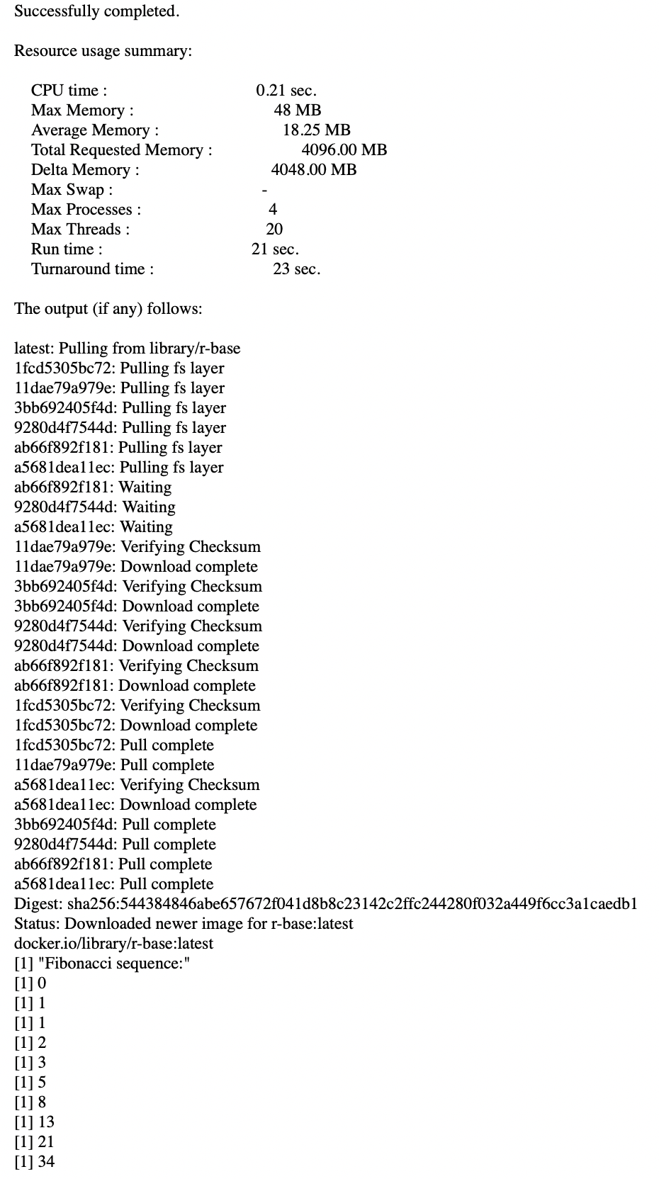
• This example shows running an R script that prints out X terms of the fibonacci sequence where X is an integer input by the user in the script.

• This type of job can also be ran as a non interactive job by changing up the bsub command slightly.

export LSF_DOCKER_VOLUMES='/path/to/storage:/path/to/storage /path/to/scratch:/path/to/scratch'

bsub -G compute-workshop -q workshop -a 'docker(r-base:latest)' Rscript /path/to/script

Adding Packages to the Docker Image

Note

• The example of Docker image building contained here assumes we are building on a local machine.

• You can build Docker images using the Compute Platform as well. That documentation can be found here.

• The first thing we need to do is determine what version of R we what to use and use that specific tag in the base docker build.

• In this process, we will be creating a Dockerfile, which can then be used by Docker to build a Docker image.

• In this case we’re going to use R 4.0.3.

#Set base image from r-base using R version 4.0.3
FROM r-base:4.0.3

• Once we have the base image decided, we need to tell the Docker file to install the packages we want.

• In the case of our example we’ll be using DeSeq2.

#Set base image from r-base using R version 4.0.3
FROM r-base:4.0.3

#Install needed R packages
RUN R -e "install.packages('DeSeq2',dependencies=TRUE, repos='http://cran.rstudio.com/')"

Note

• You can install multiple packages at the same time by adjusting the install command to the following.

RUN R -e "install.packages(c('EIAdata', 'gdata', 'ggmap', 'ggplot2'), dependencies=TRUE, repos='http://cran.studio.com/')"

• Once we save the file, we then make sure we are in the working directory that contains the Docker directory.

• Then, we can tell Docker to build this image using the following command.

docker build -t username/Dockerfile:tag directory-of-docker

Note

• username is the username of your Docker hub account.

• Dockerfile is the name you wish to give the Docker image

• tag is the tag you want to give this particular image, you can use latest or something like 1.0

  • If no tag is given, Docker will default to the latest tag, overwriting the previous image with the same name and the latest tag.

• directory-of-docker is the directory where you have saved the particular Dockerfile we are using to build the image.

• When we try to build the image using R 4.0.3, we get an error for DeSeq2.

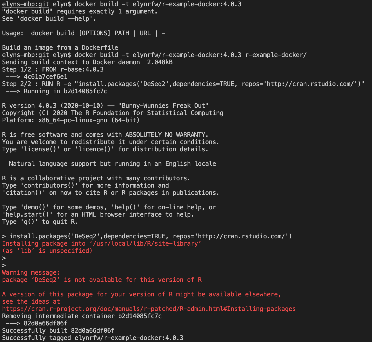
• This error is because DESeq2 is not available on CRAN, the default R packages location. It is available via Bioconductor. http://bioconductor.org/packages/release/bioc/html/DESeq2.html

Note

• There are a lot of bioinformatics packages that are not available through CRAN but are available through Bioconductor.

• To install DESeq2 we first need to install the Bioconductor manager package as this is required for Bioconductor packages.

• To do that, our updated Dockerfile code would look like the following.

#Set base image from r-base using R version 4.0.3
FROM r-base:4.0.3

#Install needed R packages
RUN R -e "install.packages('BiocManager',dependencies=TRUE, repos='http://cran.rstudio.com/')"
RUN R -e "BiocManager::install('DESeq2')"

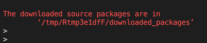
• Now when we run the docker build command, it will attempt to install the packages we’ve told it to.

• In this case that is BiocManager and all of it’s dependencies, followed by DESeq2.

• As we look at the R output the Docker gives us when attempting to build this package, we can see that an error occurs.

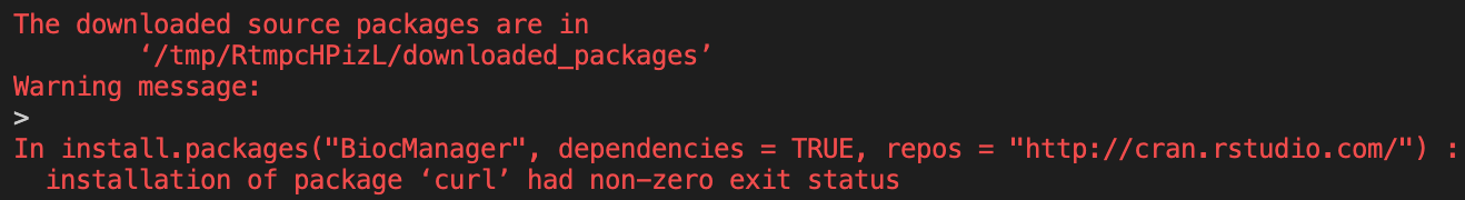
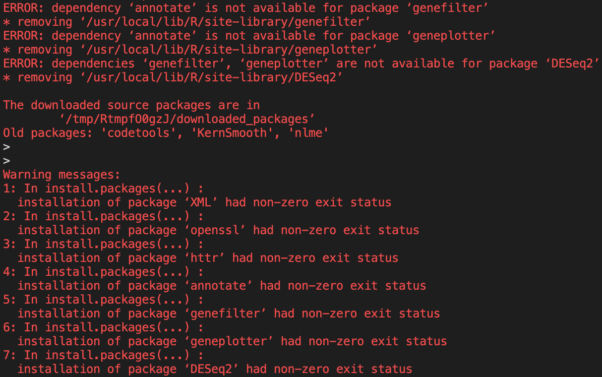
• If we look further back in the install output, we can see where this error originates.

• When the image tries to install DESeq2 we get a few errors.

• A lot of these errors look like they’re dependency errors.

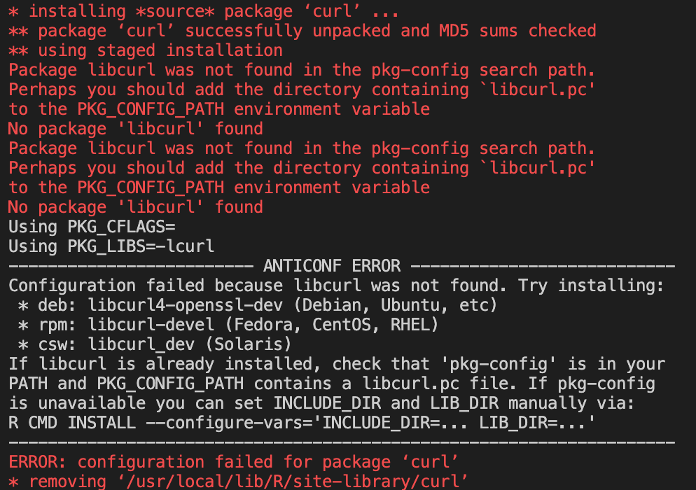
• By looking at the BiocManager error, we can see that we need to install a base OS library that’s needed for the R package.

• We can do that by adding the following code to install said library through the appropriate install method for the OS.

• The r-base Docker images use Debian as their OS, so we can install the libcurl4-openssl-dev library with apt-get.

Note

• You can find the OS version of Linux by using the cat /etc/os-release command.

#Set base image from r-base using R version 4.0.3
FROM r-base:4.0.3

#Install library dependencies
RUN apt-get update \
    && apt-get install -y --no-install-recommends libcurl4-openssl-dev \
    && apt-get clean

#Install needed R packages
RUN R -e "install.packages('BiocManager',dependencies=TRUE, repos='http://cran.rstudio.com/')"
RUN R -e "BiocManager::install('DESeq2')"

• We can rerun the docker build command with the library installed and see if that solves our issues.

• This time we will use the --no-cache option of the docker build command so that we can see if we have any install issues.

docker build --no-cache -t username/Dockerfile:tag directory-of-docker

Note

• Using the --no-cache option means that Docker will not use the cache when building the image, which means that everything will compile fresh.

• This option is not recommended all the time, only when attempting to debug an image.

• This time when the image tries to install the Curl package, it is successful.

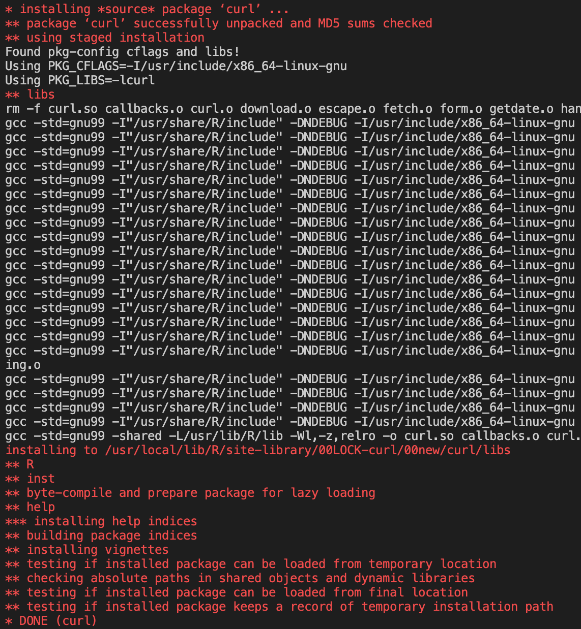
• We can also see the message at the end of the BiocManager contains no warnings.

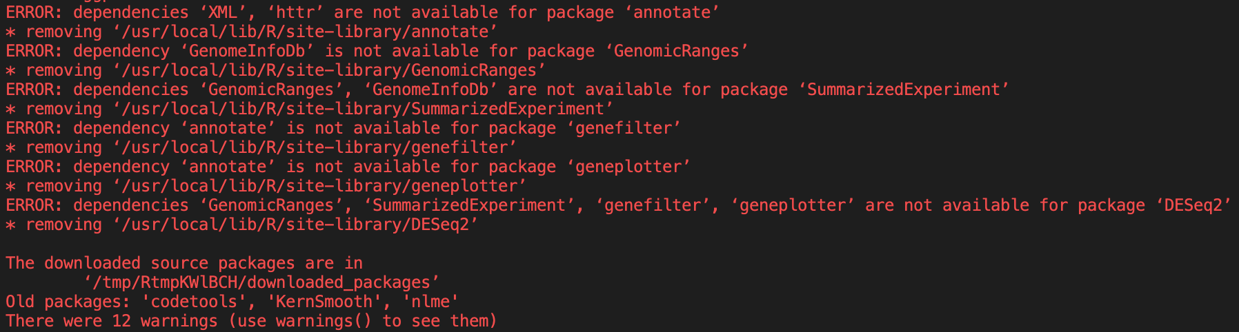
• However, DESeq2 still contains errors when it tries to install.

• If we delve into the install code, we can see that we need two more libraries based on the errors given.

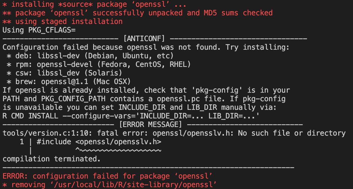
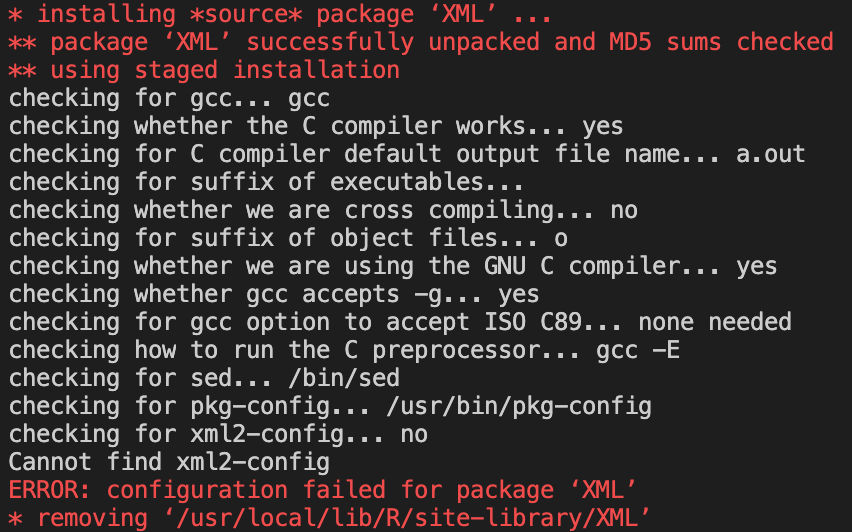
• For the first package, the error gives us the library needed, which is: libssl-dev for Debian.

• For the second package, we need to to a Google search of xml2-config as that is what the error says the package needs.

• The search results lead us to the libxml2-dev library for Debian.

• Now that we have identified which libraries we need, we can add them to the Docker file and run the build command again.

• Our Dockerfile now looks like the following.

#Set base image from r-base using R version 4.0.3
FROM r-base:4.0.3

#Install library dependencies
RUN apt-get update \
    && apt-get install -y --no-install-recommends libcurl4-openssl-dev libssl-dev libxml2-dev \
    && apt-get clean

#Install needed R packages
RUN R -e "install.packages('BiocManager',dependencies=TRUE, repos='http://cran.rstudio.com/')"
RUN R -e "BiocManager::install('DESeq2')"

• After this build attempt, we can see that we no longer have any errors the DESeq2 install either.

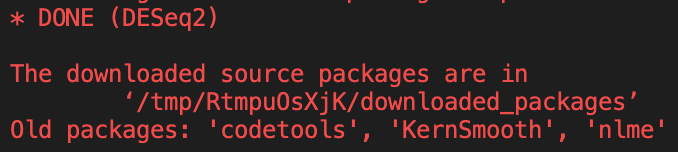
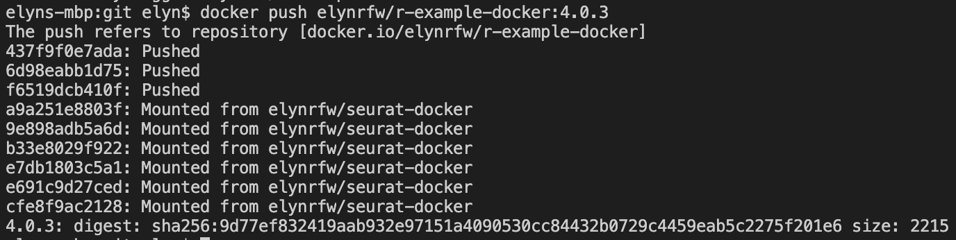
• Now that we have the R package we want to use successfully installed in a Docker image, we can push said image to our Docker Hub.

docker push username/dockerfile:tag

• Once you push the image it will be publicly available on Docker hub, unless you have changed settings.

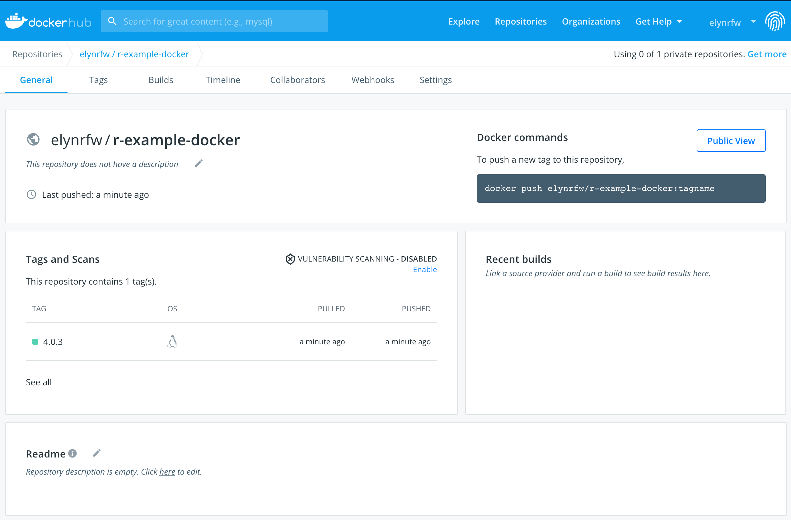
Using the R Docker Image

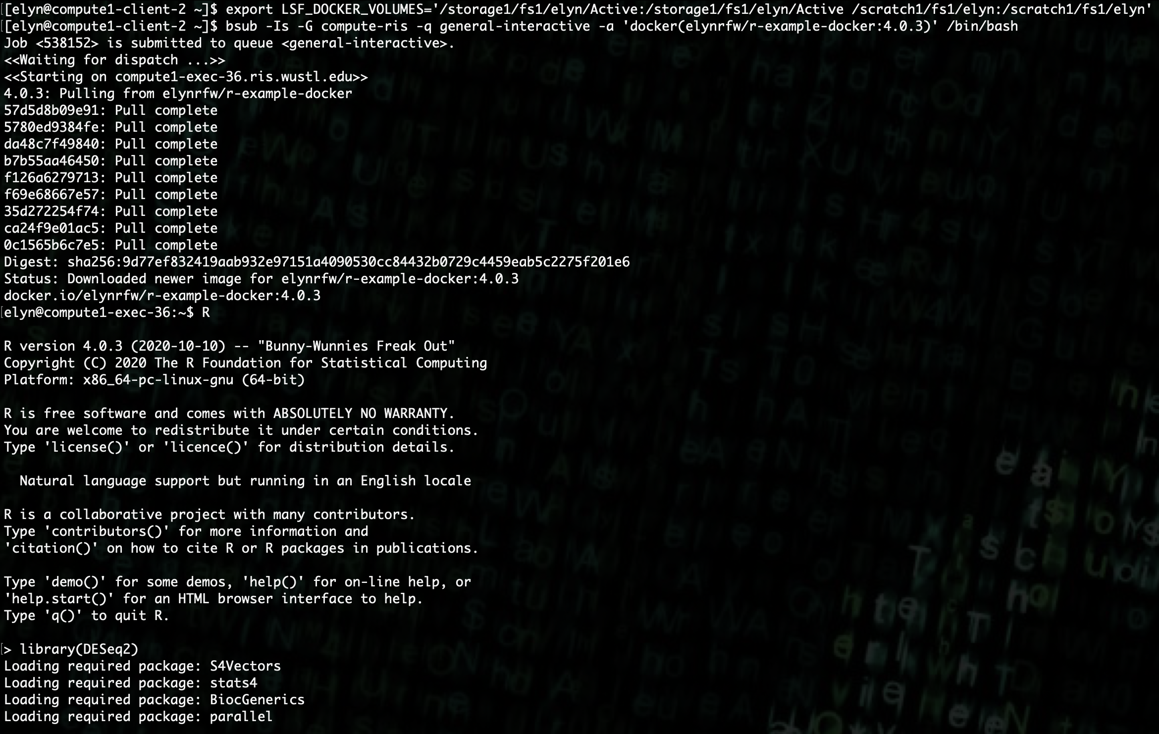
• Now that we have our Docker image upgraded and hosted on Docker hub, we can use it like we did the r-base Docker image.

export LSF_DOCKER_VOLUMES='/path/to/storage:/path/to/storage /path/to/scratch:/path/to/scratch'

bsub -Is -G compute-workshop -q workshop-interactive -a 'docker(username/dockerfile:tag)' /bin/bash

Note

• username/dockerfile:tag is the name we gave the image when we built it and pushed it to Docker hub.

Analysis Setup

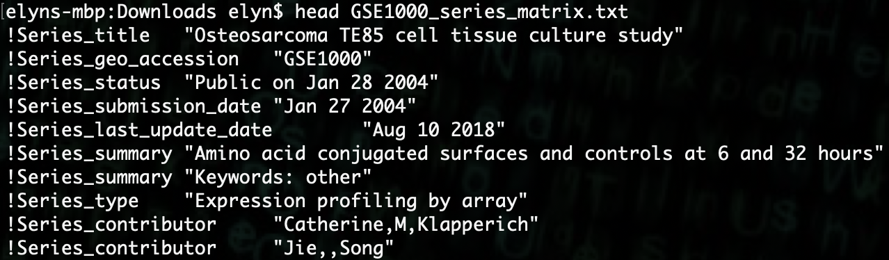
• We can now use DESeq2 to do analysis on the sample data we previously gathered.

• If we look at our data file using the linux head command, we can see that it has a lot of information at the beginning of the file.

• Each line of information starts with a !. We can remove those lines so that the file plays nice with R.

• We can use the following command to do this.

grep -v "\!" GSE1000_series_matrix.txt > GSE1000_series_matrix_fixed.txt

Note

• This file should be in the directory you will be using as the working directory for R.

• This command should be run from within the working directory. If not, you will need the full path to the file and the output.

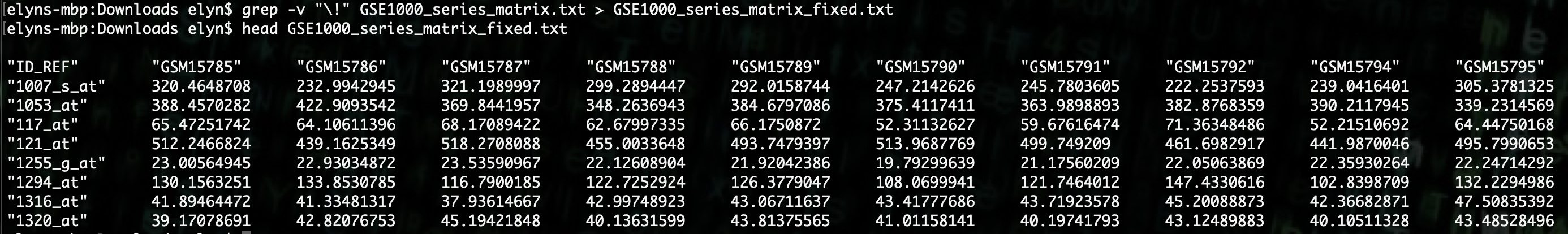
• We can now see that the file has only a single header and then a row for each sample and columns of expression data.

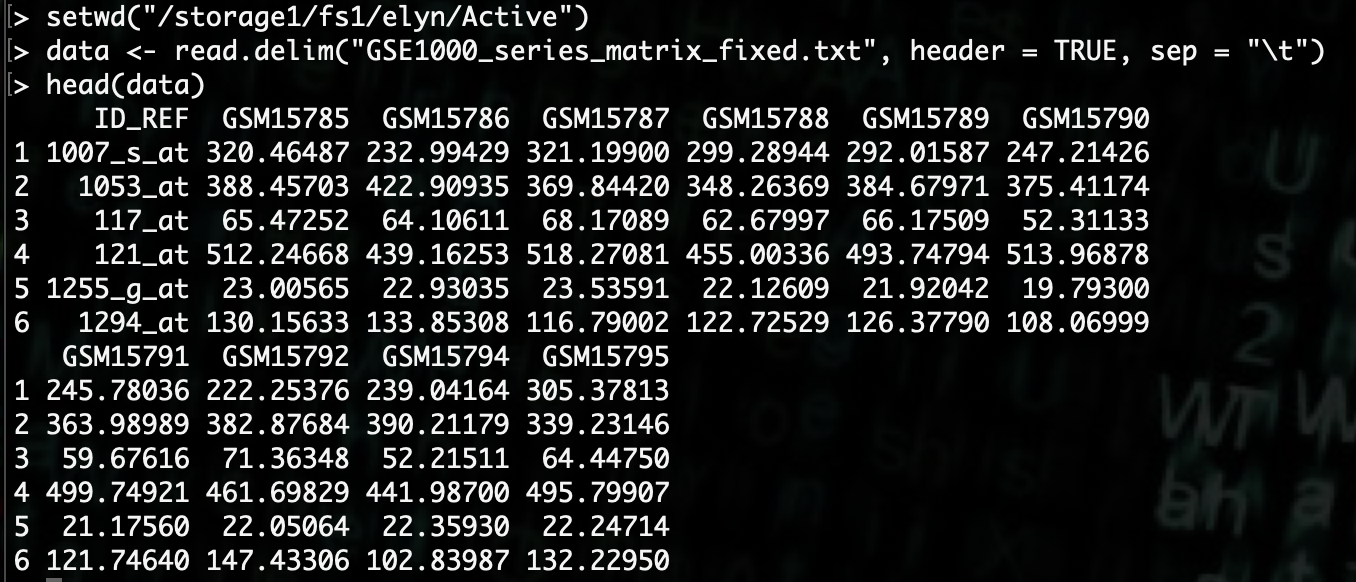
• The first thing we want to do is set our working directory and to load the data into R.

R> setwd("/path/to/storage/")
R> data <- read.delim("GSE1000_series_matrix_fixed.txt", header = TRUE, sep = "\t")

• Now that we have the data loaded, we’ll want to manipulate the data just a little bit to make it more friendly to use.

• Then we’ll set the row names to the Gene IDs and then remove that column.

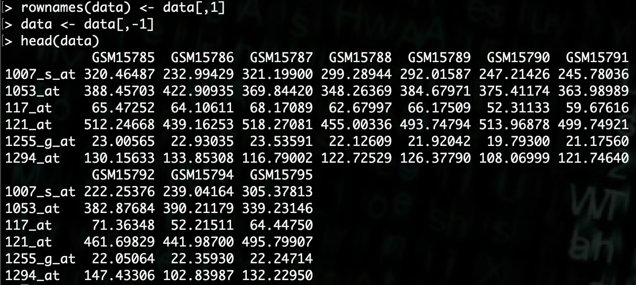
R> rownames(data) <- data[,1]
R> data <- data[,-1]

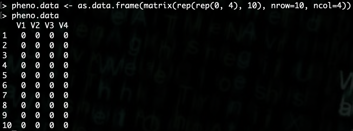
• For analysis with DESeq2 there needs to be phenotype data for the samples. Since we don’t have that available, we’ll generate some example data.

• In this dataset, there are 10 samples, so we’ll create a 10 by 4 matrix.

R> pheno.data <- as.data.frame(matrix(rep(rep(0, 4), 10), nrow=10, ncol=4))

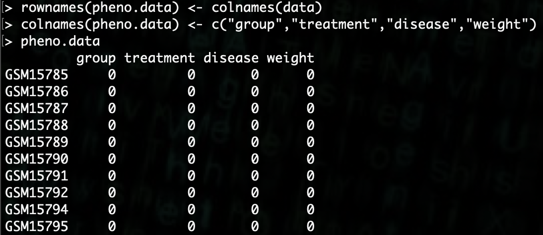
• Now that we have the dataframe created, we need to add column and row names.

R> rownames(pheno.data) <- colnames(data)
R> colnames(pheno.data) <- c("group","treatment","disease","weight")

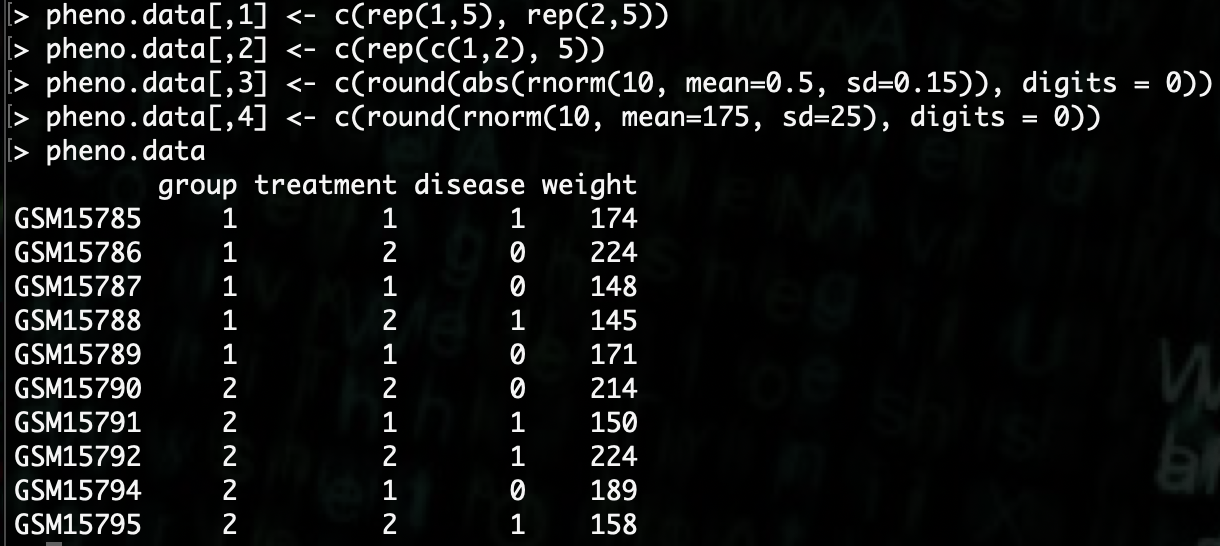
• Now we need to populate the data.

• The group data we will create 2 groups for the group column, the first group will simply be the first 5 samples and the remaining 5 will be the second group.

R> pheno.data[,1] <- c(rep(1,5), rep(2,5))

• Next we will create 2 treatments for the treatment column, we will alternate the treatments bewtween 1 and 2 regardless of group.

R> pheno.data[,2] <- c(rep(c(1,2), 5))

• Next we need to create a binary disease state of either 0 or 1. We will do this randomly.

R> pheno.data[,3] <- c(round(abs(rnorm(10, mean=0.5, sd=0.15)), digits = 0))

• Finally we will need to generate a random set of weights. We can generate those very similarly to the disease state.

R> pheno.data[,4] <- c(round(rnorm(10, mean=175, sd=25), digits = 0))

Note

• You can read more about the functions used to create the example data via the R documentation.

• rep: https://www.rdocumentation.org/packages/base/versions/3.6.2/topics/rep

• rnorm: https://www.rdocumentation.org/packages/compositions/versions/2.0-0/topics/rnorm

• abs: https://www.rdocumentation.org/packages/SparkR/versions/2.1.2/topics/abs

• round: https://www.rdocumentation.org/packages/base/versions/3.6.2/topics/Round

DESeq2 Analysis

• We now have our expression data data and our phenotypic data pheno.data, now we’re ready to analyze the data via DESeq2

• The first step is loading the DESeq2 library.

R> library(DESeq2)

Note

• The manual for DESeq2 can be found here: http://bioconductor.org/packages/release/bioc/manuals/DESeq2/man/DESeq2.pdf

• With the library loaded, we need to create a DESeq2 object that contains the data we’ve generated.

R> deseq2.data <- DESeqDataSetFromMatrix(data, pheno.data, ~ group + treatment + disease + weight)

• As we can see from the error we receive when attempting this command, our count data needs to be in integers, ie should not include decimals.

• We can fix this via the following method.

R> data <- round(data, digits = 0)

• When we do and rerun the DESeqDataSetFromMatrix command we now get a warning about our data and that certain columns of data should be designated as factors.

• We can adjust that using the following method.

R> pheno.data$group <- factor(pheno.data$group, levels = c("1","2"))
R> pheno.data$treatment <- factor(pheno.data$treatment, levels = c("1","2"))
R> pheno.data$disease <- factor(pheno.data$disease, levels = c("0","1"))

• Though this does not appear to get rid of the warning, we can continue doing analysis fine.

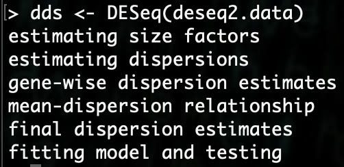
• The next step is to run the actual analysis using the DESeq() command.

R> dds <- DESeq(deseq2.data)

• Now we want to put the results into an object so that we can see what they are.

R> res <- results(dds)

• Now if we want to look at a head display of the results we can simply type the variable name res and it will give us a nice display.

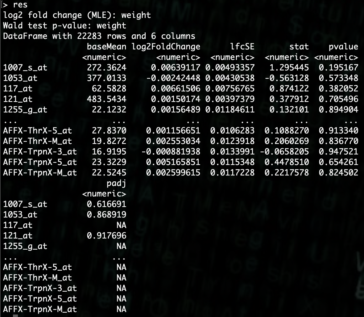
• We can see here that there are several columns for each gene that was analyzed. The column of interest for us at this point is the p-value.

• We can write a line of code using a which statement combined with the use of the dataframe signifiers to get a list of the genes that are below a certain p-value.

• First we need an object with the gene names. We can do that by using rownames and our dataset.

R> genes <- rownames(data)

• Then we create our statement to get which genes are significant at p-value < 0.01.

Note

• In this case we are selecting p < 0.01 as our signifcant threshold, but other values can be chosen.

• There are statistical methods to determine what p-value you should use, but those are not a part of this workshop.

R> significant.genes <- genes[which(res$pvalue < 0.01)]

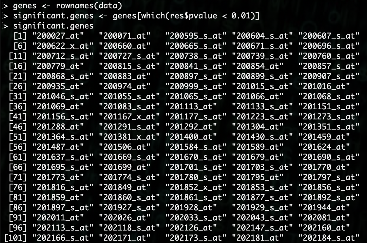
• There are a lot of genes here that are significant. We can find out how many by using the length command.

R> length(significant.genes)

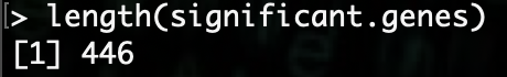
• As we can see, there are 446 genes that are significant (for this example data) based on the values we gave. We can use that data for displaying this information via graphs and charts.

Note

• You can find more information about the which and length commands at the following links.

  • which: https://www.rdocumentation.org/packages/base/versions/3.6.2/topics/which

  • length: https://www.rdocumentation.org/packages/base/versions/3.6.2/topics/length

Note

• There will be differences in the number of genes you find significant based upon the phenotype data. Since this data is randomly generated, it will change the results of the output.

• You can test this yourself by re-running the data generation steps and doing the analysis up to the length step and seeing the differences.

• You can do this until you have a workable number (~500) of significant genes to do further analysis with.

Further Analysis

• With our now identified significant genes, we can do further analysis and create graphs.

• The first thing we’ll want to do is create a data object with just the significant genes.

R> sig.data <- data[which(res$pvalue < 0.01),]

• Now we are going to look at clustering the data based off of the significant gene counts to see what that looks like.

• We will do a simple K-means clustering analysis using the kmeans command.

• But first we must transpose the dataframe for the kmeans analysis to work correctly.

R> t.sig.data <- as.data.frame(t(sig.data))
R> rownames(t.sig.data) <- colnames(sig.data)
R> colnames(t.sig.data) <- rownames(sig.data)

• We have two groups and two treatments. The first step will be to cluster into 2 groups.

R> fit2 <- kmeans(t.sig.data, 2)

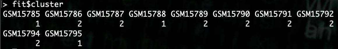
• We can look at what groups the samples got clustered into by looking at fit$cluster.

• Now we can compare that back to the original groupings by putting this information into a dataframe.

R> compare.data <- data.frame(pheno.data$group, pheno.data$treatment, pheno.data$disease, fit2$cluster)

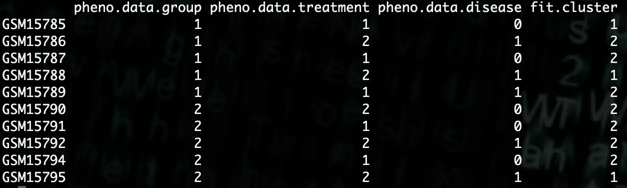
• As we can see, it does not appear to group the data based off any of our phenotypes.

• We can see if using 4 groups changes that or not.

R> fit4 <- kmeans(t.sig.data, 4)
R> compare.data2 <- data.frame(pheno.data$group, pheno.data$treatment, pheno.data$disease, fit4$cluster)

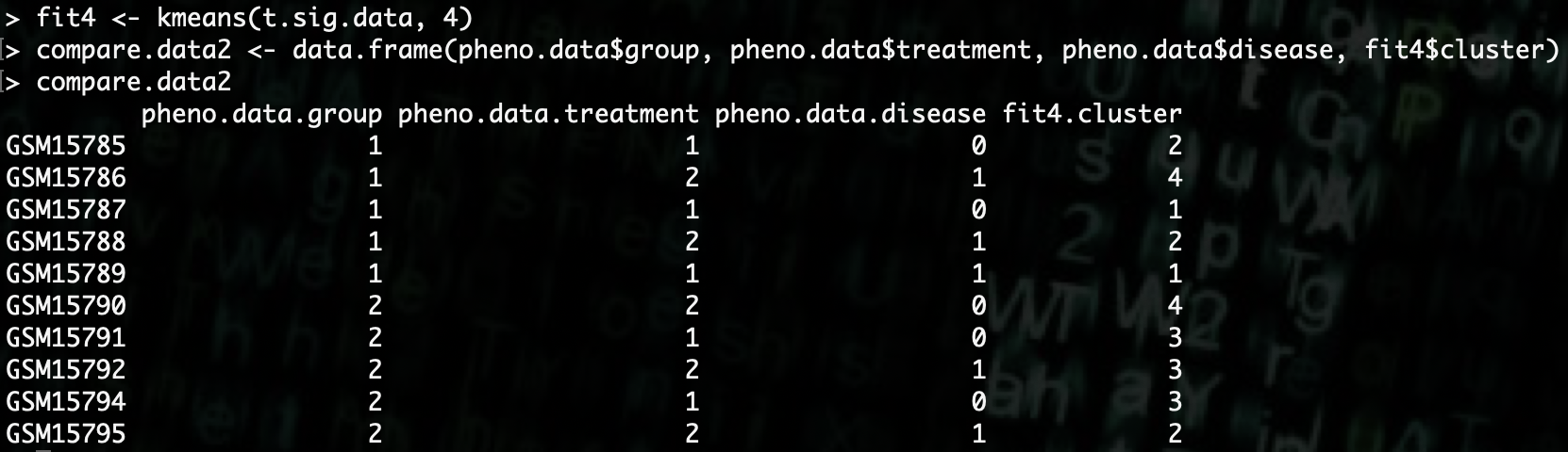
• As we can see here, using the significant genes to group the samples into 4 groups does not explain the data any better than the 2 groups.

• If we want to save the significant genes to a file, we can do that as well use the write command.

R> write(significant.genes, "significant.genes.txt")

Visualization

• You can visualize data using many different methods in R and we’ll go through a couple of examples.

Note

Because of the way jobs run on the server and given the visualization limitations of ssh connections, most methods will have to output the visualization directly to a file.

• The first thing we’re going to start off with is a simple bar chart. We’ll create one based off the first significant gene.

R> barplot(t.sig.data[,1], main="Gene 1", xlab="Counts", names.arg=rownames(t.sig.data))

• This is simply the command to create a bar plot, now we have to make it so that it prints the plot to a file

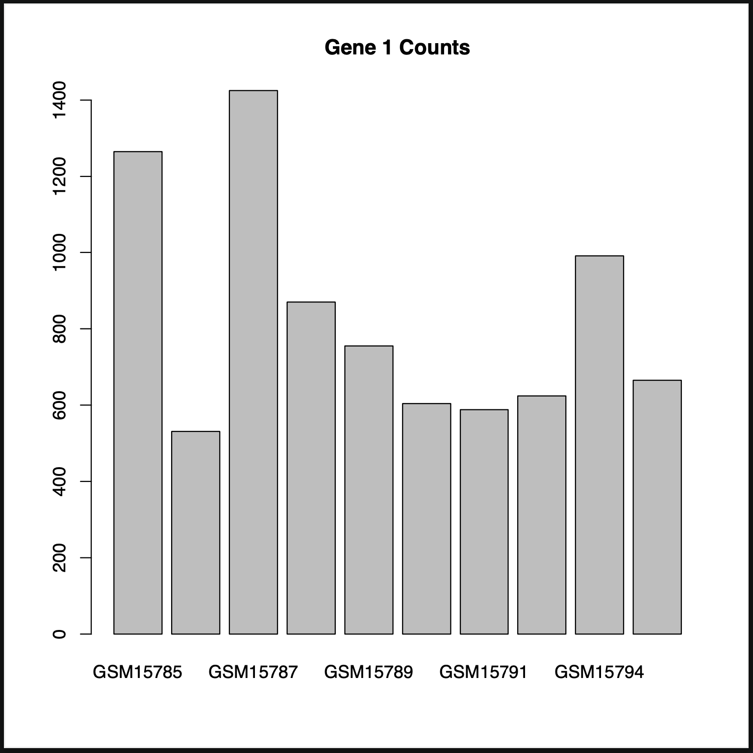
R> pdf("gene1.pdf")
R> barplot(t.sig.data[,1], main="Gene 1 Counts", names.arg=rownames(t.sig.data))
R> dev.off()

• As we can see, it generates a pdf that has our graph.

• If we look at the graph, we can see that some of the names aren’t displayed as they’re rather long, we can adjust this with a couple of options.

  • The first is to rotate the names with the las option.

  • The second is to adjust the margin using the parameter command par().

  • The third is to adjust the height on the pdf. The default is 7.

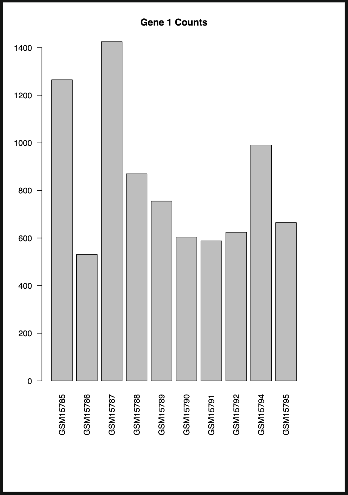
R> pdf("gene1.pdf", height=10)
R> par(mar=c(11,4,4,4))
R> barplot(t.sig.data[,1], main="Gene 1 Counts", names.arg=rownames(t.sig.data), las=2)
R> dev.off()

• Given that we can have multiple, and possibly hundreds of genes that we may want to create a graph for, we can use a for loop in R to loop through the genes.

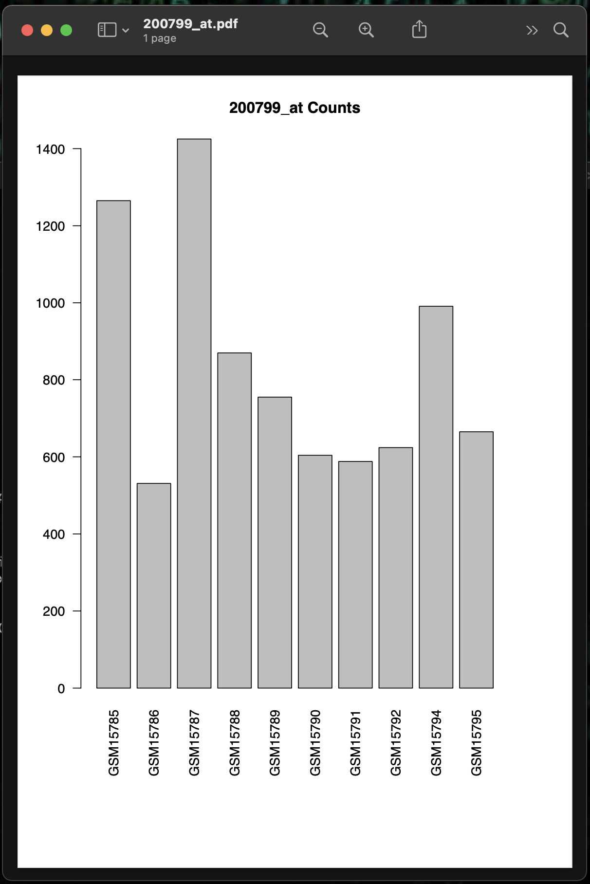
• The first thing we’ll need to do is adjust the commands to use the names of the genes for the pdf file and for the graph title.

R> pdf(paste(significant.genes[1], ".pdf", sep=""), height=10)
R> par(mar=c(11,4,4,4))
R> barplot(t.sig.data[,1], main=paste(significant.genes[1], "Counts", sep=" "), names.arg=rownames(t.sig.data), las=2)
R> dev.off()

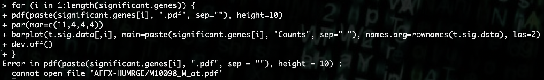
• Now that we have that setup, we can introduce the for loop so that it loops through all the significant genes.

R> for (i in 1:length(significant.genes)) {
R> pdf(paste(significant.genes[i], ".pdf", sep=""), height=10)
R> par(mar=c(11,4,4,4))
R> barplot(t.sig.data[,i], main=paste(significant.genes[i], "Counts", sep=" "), names.arg=rownames(t.sig.data), las=2)
R> dev.off()
R> }

• When we run this, we get an error because there are special characters in the gene name that Linux does not like in file names.

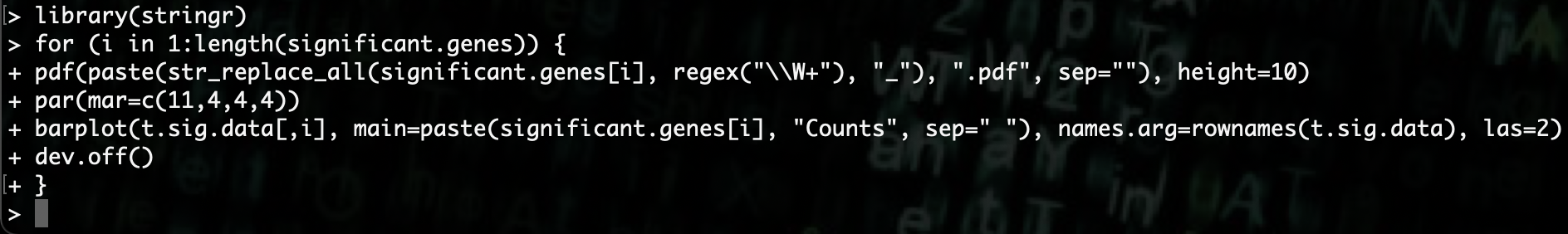
• To correct this, we can use the str_replace_all command combined with a regular expression to replace all non alphanumberic characters with and underscore.

• This command is part of the stringr library.

R> library(stringr)
R> str_replace_all(significant.genes[i], regex("\\W+"), "_")

• Once we add that to our for loop, we see that we no longer get the error.

R> for (i in 1:length(significant.genes)) {
R> pdf(paste(str_replace_all(significant.genes[i], regex("\\W+"), "_"), ".pdf", sep=""), height=10)
R> par(mar=c(11,4,4,4))
R> barplot(t.sig.data[,i], main=paste(significant.genes[i], "Counts", sep=" "), names.arg=rownames(t.sig.data), las=2)
R> dev.off()
R> }

• If we look in the working directory, we can see that we have a list of graphs of all the genes that are significant.

• You can put all of these commands into one R script.

#Set the working directory
setwd("/path/to/working/directory")

#Load the Libraries
library(DESeq2)
library(stringr)

#Read the Expression Data into an Object
data <- read.delim("GSE1000_series_matrix_fixed.txt", header = TRUE, sep = "\t")

#Rename the row names with the Gene IDs and remove the Gene ID row
rownames(data) <- data[,1]
data <- data[,-1]
data <- round(data, digits = 0)

#Create a data frame for the create phenotype data
pheno.data <- as.data.frame(matrix(rep(rep(0, 4), 10), nrow=10, ncol=4))

#Give the row and column names the appropriate sample and phenotype names
rownames(pheno.data) <- colnames(data)
colnames(pheno.data) <- c("group","treatment","disease","weight")

#Populate the phenotype data frame
pheno.data[,1] <- c(rep(1,5), rep(2,5))
pheno.data[,2] <- c(rep(c(1,2), 5))
pheno.data[,3] <- c(round(abs(rnorm(10, mean=0.5, sd=0.15)), digits = 0))
pheno.data[,4] <- c(round(rnorm(10, mean=175, sd=25), digits = 0))

#Fixing the phenotype data
pheno.data$group <- factor(pheno.data$group, levels = c("1","2"))
pheno.data$treatment <- factor(pheno.data$treatment, levels = c("1","2"))
pheno.data$disease <- factor(pheno.data$disease, levels = c("0","1"))

#Creating the DESeq2 object
deseq2.data <- DESeqDataSetFromMatrix(data, pheno.data, ~ group + treatment + disease + weight)

#Running the DESeq2 analysis
dds <- DESeq(deseq2.data)

#Getting Results
res <- results(dds)
genes <- rownames(data)
significant.genes <- genes[which(res$pvalue < 0.01)]

#Getting the significant genes
sig.data <- data[which(res$pvalue < 0.01),]

#Doing K-means clustering analysis
t.sig.data <- as.data.frame(t(sig.data))
rownames(t.sig.data) <- colnames(sig.data)
colnames(t.sig.data) <- rownames(sig.data)
fit2 <- kmeans(t.sig.data, 2)
compare.data <- data.frame(pheno.data$group, pheno.data$treatment, pheno.data$disease, fit2$cluster)
fit4 <- kmeans(t.sig.data, 4)
compare.data2 <- data.frame(pheno.data$group, pheno.data$treatment, pheno.data$disease, fit4$cluster)

#Writing the list of significant genes to a file
write(significant.genes, "significant.genes.txt")

#Visualization of data

#Bar Plot
pdf("gene1.pdf", height=10)
par(mar=c(11,4,4,4))
barplot(t.sig.data[,1], main="Gene 1 Counts", names.arg=rownames(t.sig.data), las=2)
dev.off()

for (i in 1:length(significant.genes)) {
pdf(paste(str_replace_all(significant.genes[i], regex("\\W+"), "_"), ".pdf", sep=""), height=10)
par(mar=c(11,4,4,4))
barplot(t.sig.data[,i], main=paste(significant.genes[i], "Counts", sep=" "), names.arg=rownames(t.sig.data), las=2)
dev.off()
}

Running an R-script

• If we put the previous into a file and call it example.R, we have created an R-script that we can run without having to go into R.

• The R-script can be run either interactively or a non-interactive job.

export LSF_DOCKER_VOLUMES='/path/to/storage:/path/to/storage /path/to/scratch:/path/to/scratch'
bsub -Is -G compute-workshop -q workshop-interactive -a 'docker(username/dockerfile:tag)' Rscript /path/to/example.R

export LSF_DOCKER_VOLUMES='/path/to/storage:/path/to/storage /path/to/scratch:/path/to/scratch'
bsub -G compute-workshop -q workshop -a 'docker(username/dockerfile:tag)' Rscript /path/to/example.R

• We start with just the sample data file in our working directory.

• Then we run the R-script with an interactive command.

• And now we can see that we have graphs of the significant genes as pdf files, and the list of significant genes in the file: significant.genes.txt.

Note

• We will be covering Rstudio in another workshop.